Home-to-work commuting flows within the municipalities around Paris
Source:vignettes/paris_commute_flows.Rmd
paris_commute_flows.RmdIntroduction
This article illustrates the use of the spflow
package for modeling spatial interactions using the example of
home-to-work commuting flows. For our example we use information on the
71 municipalities that are located closest to the center of Paris. This
data is contained in the package and was originally diffused by the
French National Institutes of Statistics and Economic Studies (INSEE),
and of Geographic and Forest Information (IGN). (For more information
see help(paris_data).)
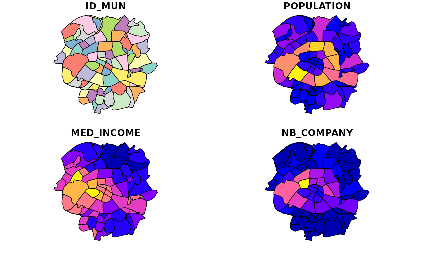
Data presentation
Each municipality is identified by a unique id. Additionally, we have information on the population, the median income and the number of companies.
There are three different neighborhood matrices that can be used to describe the connectivity between the municipalities.
old_par <- par(mfrow = c(1, 3), mar = c(0,0,1,0))

mid_points <- suppressWarnings({
    st_point_on_surface(st_geometry(paris10km_municipalities))})

paris10km_nb <- list(
  "by_contiguity" = spdep::poly2nb(paris10km_municipalities),
  "by_distance" = spdep::dnearneigh(mid_points,d1 = 0, d2 = 5),
  "by_knn" = spdep::knn2nb(knearneigh(mid_points,3))
)

plot(st_geometry(paris10km_municipalities))
plot(paris10km_nb$by_contiguity, mid_points, add = T, col = rgb(0,0,0,alpha=0.5))
title("Contiguity")

plot(st_geometry(paris10km_municipalities))
plot(paris10km_nb$by_distance,mid_points, add = T, col = rgb(0,0,0,alpha=0.5))
title("Distance")

plot(st_geometry(paris10km_municipalities))
plot(paris10km_nb$by_knn, mid_points, add = T, col = rgb(0,0,0,alpha=0.5))
title("3 Nearest Neighbors")

par(old_par)
Finally, there is data on the size of the commuting flows and the distance between all pairs of municipalities
head(paris10km_commuteflows)
#>   ID_ORIG ID_DEST DISTANCE COMMUTE_FLOW
#> 1   75101   75101    0.000   3771.23556
#> 2   75101   75102  786.743    294.76899
#> 3   75101   75103 1729.063     71.25116
#> 4   75101   75104 1807.294     99.38468
#> 5   75101   75105 2266.598     98.88915
#> 6   75101   75106 1512.870     65.15406
Modeling Spatial Interactions with spflow()
The spflow package builds on the idea that flows correspond to pairwise interactions between the nodes of an origin network with the nodes of a destination network.
In our example, the origin and destination networks are the same because every municipality is both an origin and destination of a flow.
To estimate the model efficiently, the spflow package uses moment-based estimation methods, that exploit the relational structure of flow data. This avoids duplication arising from the fact that each municipality is at the origin and destination of many flows. For more details on the model and the estimation methods see LeSage (2008), Dargel (2021) and Dargel (2022).
The spflow network objects
To describe the nodes of a network the package provides
spflow_network-class that combines attributes of the nodes
with the chosen network structure. For our model we choose the
contiguity based neighborhood structure.
paris10km_net <- spflow_network(
    id_net = "paris",
    node_neighborhood = nb2mat(paris10km_nb$by_contiguity),
    node_data = paris10km_municipalities,
    node_key_column = "ID_MUN")

paris10km_net
#> Spatial network nodes with id: paris
#> --------------------------------------------------
#> Number of nodes: 71
#> Average number of links per node: 5.239
#> Density of the neighborhood matrix: 7.38% (non-zero connections)
#>
#> Data on nodes:
#>     ID_MUN POPULATION MED_INCOME NB_COMPANY AREA COORD_X COORD_Y
#> 1    75101      17100   31842.56      14333  182    2.34   48.86
#> 2    75102      22390    30024.5      14478   99    2.34   48.87
#> 3    75103      35991      30988      10696  117    2.36   48.86
#> 4    75104      27769   30514.67       7412  160    2.36   48.85
#> 5    75105      60179      32950      10290  252    2.35   48.85
#> 6    75106      43224   38447.69      10620  215    2.33   48.85
#> ---    ---        ---        ---        ---  ---     ---     ---
#> 66   94046      54186      24329       3385  537    2.44    48.8
#> 67   94067      21846   31559.38       1763   90    2.42   48.84
#> 68   94069      14870   25790.65        957  144    2.43   48.82
#> 69   94076      56504      19447       2690  529    2.36   48.79
#> 70   94080      49831      30798       4655  191    2.43   48.85
#> 71   94081      88102    17860.5       4467 1166     2.4   48.79
The spflow_network_pair-class contains all information
on the pairs of nodes belonging to the origin and destination
networks.
paris10km_net_pairs <- spflow_network_pair(
  id_orig_net = "paris",
  id_dest_net = "paris",
  pair_data = paris10km_commuteflows,
  orig_key_column = "ID_ORIG",
  dest_key_column = "ID_DEST")

paris10km_net_pairs
#> Spatial network pair with id: paris_paris
#> --------------------------------------------------
#> Origin network id: paris (with 71 nodes)
#> Destination network id: paris (with 71 nodes)
#> Number of pairs: 5041
#> Completeness of pairs: 100.00% (5041/5041)
#>
#> Data on node-pairs:
#>      ID_DEST ID_ORIG DISTANCE COMMUTE_FLOW
#> 1      75101   75101        0      3771.24
#> 2      75102   75101   786.74       294.77
#> 3      75103   75101  1729.06        71.25
#> 4      75104   75101  1807.29        99.38
#> 5      75105   75101   2266.6        98.89
#> 6      75106   75101  1512.87        65.15
#> ---      ---     ---      ---          ---
#> 5036   94046   94081  3742.08       218.66
#> 5037   94067   94081  6105.73        60.28
#> 5038   94069   94081  4535.03       102.04
#> 5039   94076   94081  2567.25      1067.62
#> 5040   94080   94081  7277.43       120.11
#> 5041   94081   94081        0      9257.91
The spflow_network_multi-class combines information on
the nodes and the node-pairs and also ensures that both data sources are
consistent. For example, if some of the origins in the
spflow_network_pair-class are not identified with the nodes
in the spflow_network-class an error will be raised.
paris10km_multinet <- spflow_network_multi(paris10km_net,paris10km_net_pairs)
paris10km_multinet
#> Collection of spatial network nodes and pairs
#> --------------------------------------------------
#> Contains 1 spatial network nodes
#>     With id :  paris
#> Contains 1 spatial network pairs
#>     With id :  paris_paris
#>
#> Availability of origin-destination pair information:
#>
#>  ID_ORIG_NET ID_DEST_NET ID_NET_PAIR COMPLETENESS   C_PAIRS C_ORIG C_DEST
#>        paris       paris paris_paris      100.00% 5041/5041  71/71  71/71
Given the information on origins, destinations and OD pairs we can
use the spflow_map() method for a simple geographic
representation of the largest flows.
plot(paris10km_municipalities$geometry) # polygons as background
spflow_map(
  paris10km_multinet,
  flow_var = "COMMUTE_FLOW",
  add = TRUE,          # add to existing background
  legend_position = "bottomleft",
  filter_lowest = .95, # concentrate on the 5% largest
  remove_intra = TRUE,  # intra-municipality flows are too large
  cex = 1)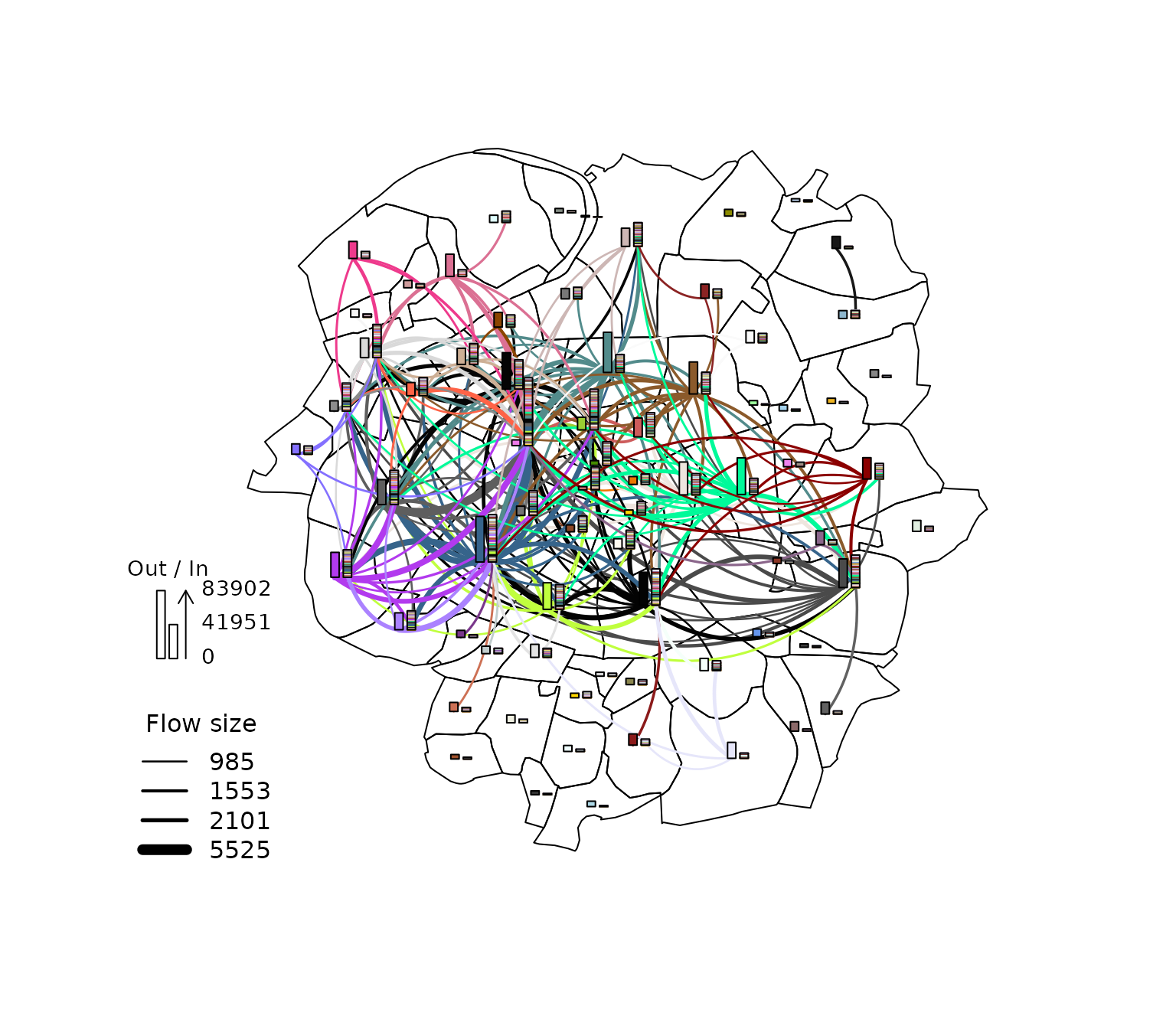
Before estimating a model we should investigate the correlation
structure of the input data. The pair_cor() method creates
a correlation matrix, which we can represent using the
cor_image(). The formula is used clarify which variables
should be included in the correlation matrix. The details of how to use
this formula are explained later in this vignette and documented in
?spflow.
cor_formula <- log(1 + COMMUTE_FLOW) ~ . + P_(log( 1 + DISTANCE))
cor_mat <- pair_cor(paris10km_multinet, spflow_formula = cor_formula, add_lags_x = FALSE)

colnames(cor_mat) <- paste0(substr(colnames(cor_mat),1,3),"...") #truncate top labels
cor_image(cor_mat)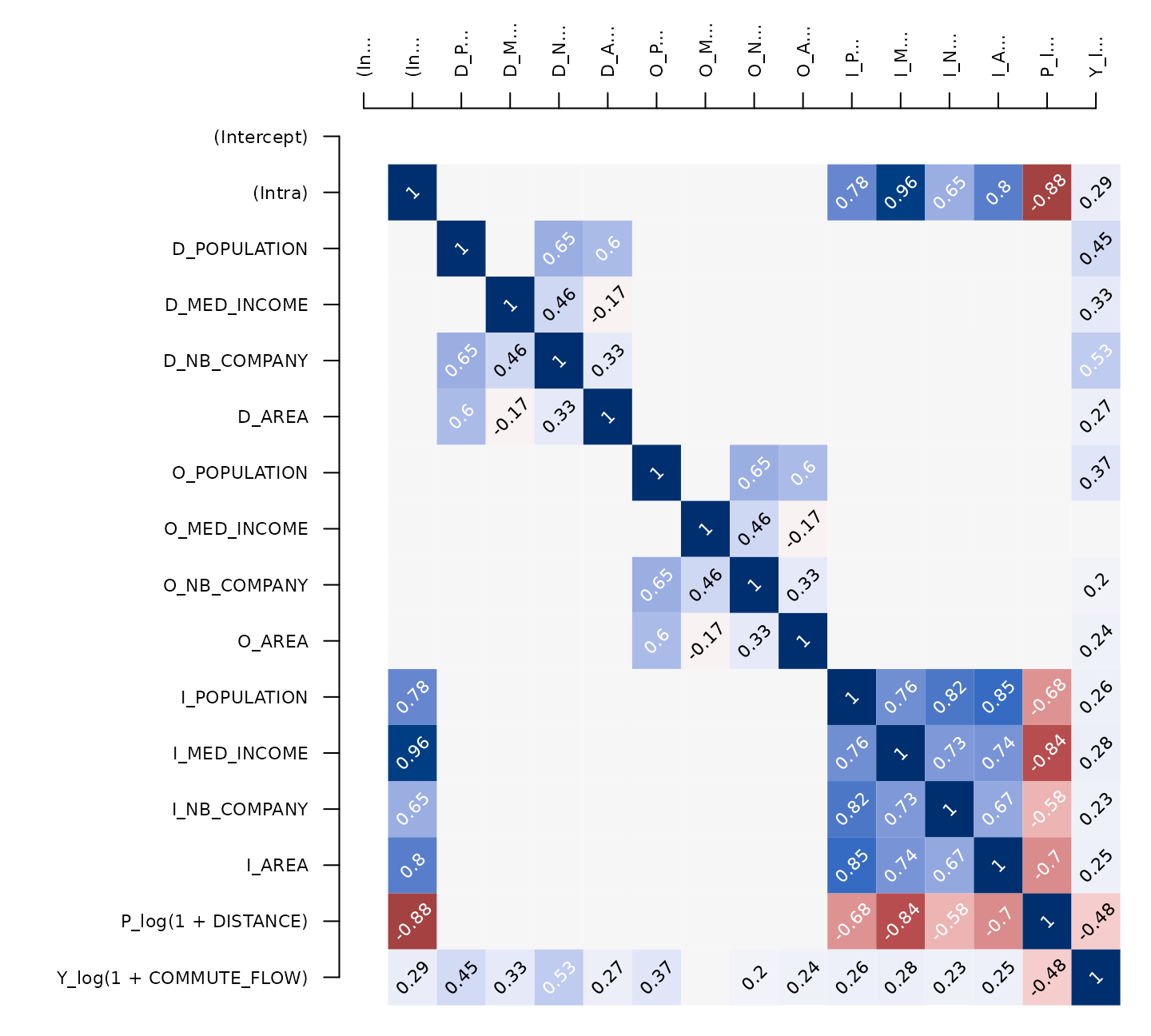
Estimation
The core function of the package is spflow(), which
provides an interface to four different estimators of the spatial
econometric interaction model.
Estimating with default values
Estimation with default settings requires two arguments: a
spflow_network_multi-class and a
spflow_formula. The spflow_formula specifies
the model we want to estimate. In this example, the dependent variable
is a transformation of commuting flows and we use the do- shortcut to
indicate that all available variables should be included in the model.
Using the defaults leads to the most comprehensive spatial interaction
model, which includes spatial lags of the dependent variable, the
exogenous variables and additional attributes for intra-regional
observations.
results_default <- spflow(
  spflow_formula = log(1 + COMMUTE_FLOW) ~ . + P_(log( 1 + DISTANCE)),
  spflow_networks = paris10km_multinet)

results_default
#> --------------------------------------------------
#> Spatial interaction model estimated by: MLE
#> Spatial correlation structure: SDM (model_9)
#> Dependent variable: log(1 + COMMUTE_FLOW)
#>
#> --------------------------------------------------
#> Coefficients:
#>                         est     sd   t.stat  p.val
#> rho_d                 0.439  0.016   27.833  0.000
#> rho_o                 0.796  0.010   82.407  0.000
#> rho_w                -0.372  0.020  -18.225  0.000
#> (Intercept)          -0.158  0.073   -2.168  0.030
#> (Intra)               6.180  0.296   20.908  0.000
#> D_POPULATION          0.000  0.000    4.254  0.000
#> D_POPULATION.lag1     0.000  0.000   -0.170  0.865
#> D_MED_INCOME          0.000  0.000   -2.422  0.015
#> D_MED_INCOME.lag1     0.000  0.000    6.300  0.000
#> D_NB_COMPANY          0.000  0.000    2.437  0.015
#> D_NB_COMPANY.lag1     0.000  0.000    2.542  0.011
#> D_AREA                0.000  0.000    6.368  0.000
#> D_AREA.lag1           0.000  0.000   -4.319  0.000
#> O_POPULATION          0.000  0.000   22.903  0.000
#> O_POPULATION.lag1     0.000  0.000   -5.740  0.000
#> O_MED_INCOME          0.000  0.000    0.609  0.542
#> O_MED_INCOME.lag1     0.000  0.000    0.192  0.848
#> O_NB_COMPANY          0.000  0.000   -5.610  0.000
#> O_NB_COMPANY.lag1     0.000  0.000    1.050  0.294
#> O_AREA                0.000  0.000    6.278  0.000
#> O_AREA.lag1           0.000  0.000   -4.952  0.000
#> I_POPULATION          0.000  0.000   -3.539  0.000
#> I_MED_INCOME          0.000  0.000   -8.722  0.000
#> I_NB_COMPANY          0.000  0.000    4.787  0.000
#> I_AREA               -0.001  0.000   -5.402  0.000
#> P_log(1 + DISTANCE)      NA     NA       NA     NA
#>
#> --------------------------------------------------
#> R2_corr: 0.9110002
#> Observations: 5041
#> Model coherence: Validated
Adjusting the formula
We can adjust how the exogenous variables are to be used by wrapping
them into the D_(), O_(), I_()
and P_() functions. The variables in P_() are
used as OD pair features and those in D_(),
O_() and I_() are used as destination, origin
and intra-regional features. We can take advantage of the formula
interface to specify transformations and expand factor variables to
dummies.
clog <- function(x) {
  log_x <- log(x)
  log_x - mean(log_x)
}

spflow_formula  <-
  log(COMMUTE_FLOW + 1) ~
  D_(log(NB_COMPANY) + clog(MED_INCOME)) +
  O_(log(POPULATION) + clog(MED_INCOME)) +
  I_(log(POPULATION)) +
  P_(log(DISTANCE + 1))

results_mle  <- spflow(
  spflow_formula,
  paris10km_multinet)
results_mle
#> --------------------------------------------------
#> Spatial interaction model estimated by: MLE
#> Spatial correlation structure: SDM (model_9)
#> Dependent variable: log(COMMUTE_FLOW + 1)
#>
#> --------------------------------------------------
#> Coefficients:
#>                             est     sd   t.stat  p.val
#> rho_d                     0.213  0.019   11.150  0.000
#> rho_o                     0.726  0.012   59.127  0.000
#> rho_w                    -0.022  0.024   -0.904  0.366
#> (Intercept)              -0.809  0.289   -2.796  0.005
#> (Intra)                   6.829  0.893    7.646  0.000
#> D_log(NB_COMPANY)         0.285  0.016   18.075  0.000
#> D_log(NB_COMPANY).lag1   -0.220  0.022  -10.099  0.000
#> D_clog(MED_INCOME)       -0.343  0.051   -6.663  0.000
#> D_clog(MED_INCOME).lag1   0.509  0.073    6.959  0.000
#> O_log(POPULATION)         0.763  0.021   36.230  0.000
#> O_log(POPULATION).lag1   -0.649  0.031  -21.085  0.000
#> O_clog(MED_INCOME)       -0.081  0.050   -1.631  0.103
#> O_clog(MED_INCOME).lag1  -0.006  0.066   -0.094  0.925
#> I_log(POPULATION)        -0.422  0.082   -5.178  0.000
#> P_log(DISTANCE + 1)      -0.073  0.022   -3.257  0.001
#>
#> --------------------------------------------------
#> R2_corr: 0.9207572
#> Observations: 5041
#> Model coherence: Validated
Fine-grained control with spflow_control()
More fine-grained adjustments are possible via the
spflow_control argument. Here we change the estimation
method and the way we want to model the spatial autoregression in the
flows. To use spatial lags only for certain variables, we need to
specify them as a second formula.
sdm_formula <- ~
  O_(log(POPULATION) + clog(MED_INCOME)) +
  D_(log(NB_COMPANY) + clog(MED_INCOME))

cntrl <- spflow_control(
  estimation_method = "mcmc",
  sdm_variables = sdm_formula,
  model = "model_7") # restricts \rho_w = 0

results_mcmc  <- spflow(
  spflow_formula,
  paris10km_multinet,
  estimation_control = cntrl)

results_mcmc
#> --------------------------------------------------
#> Spatial interaction model estimated by: MCMC
#> Spatial correlation structure: SDM (model_7)
#> Dependent variable: log(COMMUTE_FLOW + 1)
#>
#> --------------------------------------------------
#> Coefficients:
#>                             est  quant_025  quant_975     sd
#> rho_d                     0.200      0.172      0.227  0.014
#> rho_o                     0.723      0.698      0.745  0.012
#> (Intercept)              -0.768     -1.326     -0.201  0.281
#> (Intra)                   6.812      5.036      8.560  0.908
#> D_log(NB_COMPANY)         0.290      0.259      0.321  0.016
#> D_log(NB_COMPANY).lag1   -0.229     -0.267     -0.191  0.019
#> D_clog(MED_INCOME)       -0.346     -0.447     -0.243  0.052
#> D_clog(MED_INCOME).lag1   0.507      0.365      0.651  0.073
#> O_log(POPULATION)         0.776      0.743      0.810  0.017
#> O_log(POPULATION).lag1   -0.667     -0.713     -0.621  0.024
#> O_clog(MED_INCOME)       -0.083     -0.178      0.014  0.050
#> O_clog(MED_INCOME).lag1  -0.003     -0.131      0.126  0.066
#> I_log(POPULATION)        -0.420     -0.583     -0.257  0.083
#> P_log(DISTANCE + 1)      -0.070     -0.113     -0.030  0.022
#>
#> --------------------------------------------------
#> R2_corr: 0.920582
#> Observations: 5041
#> Model coherence: Validated
Visualisations to diagnose the fit
Calling plot(results_mcmc) would create a whole sequence
of graphics that allow to diagnose the fit. Here we concentrate on a
selection of these graphics. The pairwise correlations of the model data
show, for example, that the residuals and their spatial lags are not
correlated with the explanatory variables.
res_corr <- pair_cor(results_mcmc)
colnames(res_corr) <- substr(colnames(res_corr),1,3)
cor_image(res_corr)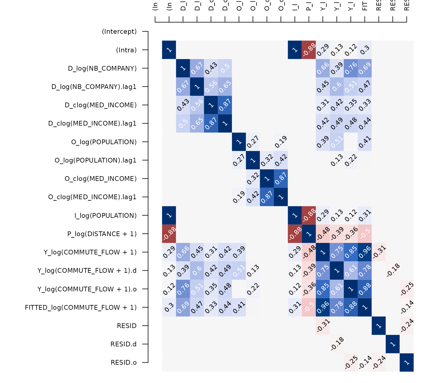
We can also create Moran scatter plots to check whether the residuals still exhibit spatial autocorrelation with respect to the three potential neighborhood matrices \(W_d\), \(W_o\) and \(W_w\).
old_par <- par(mfrow = c(1, 3), mar = c(2,2,2,2))
spflow_moran_plots(results_mcmc)
par(old_par)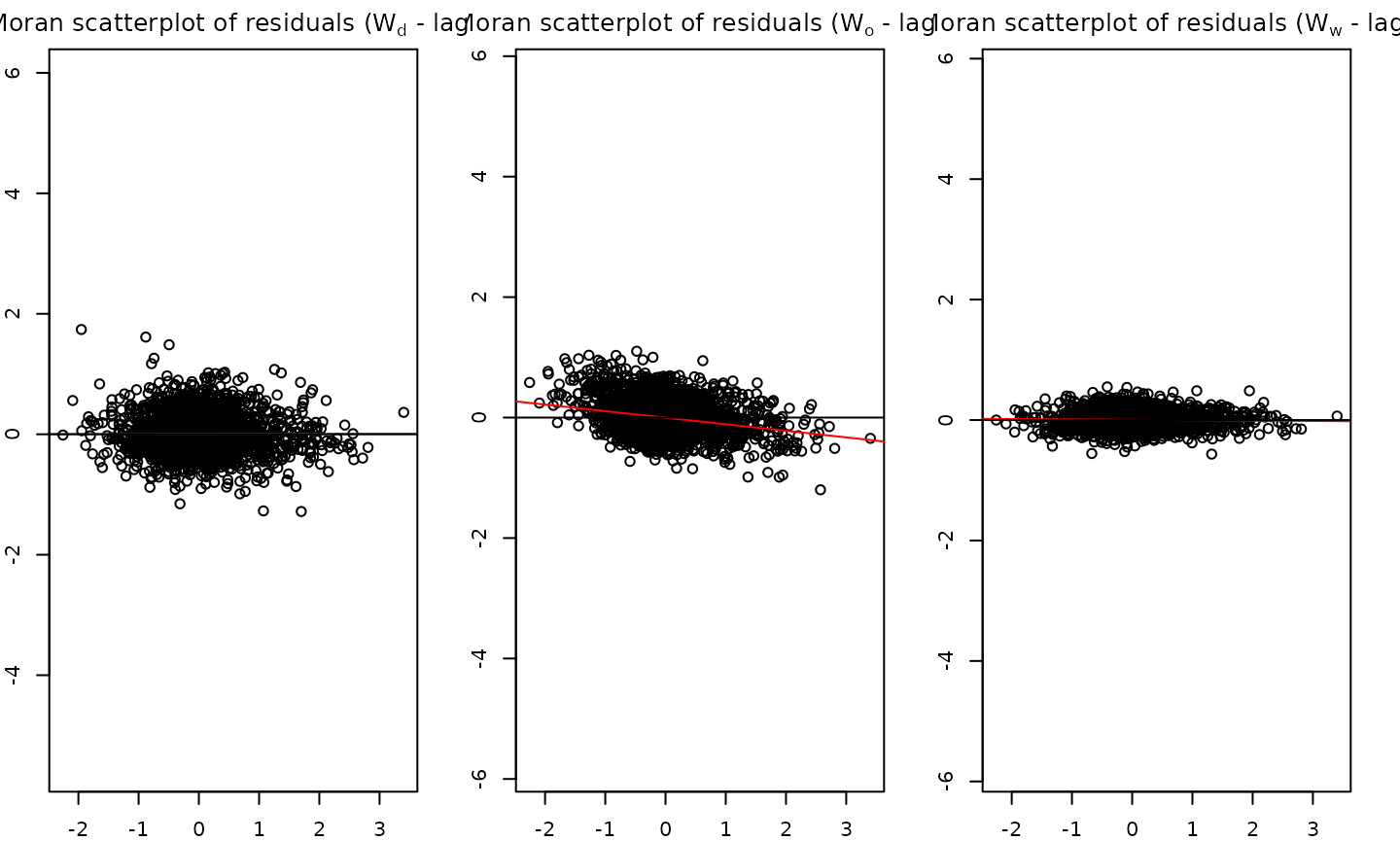
A quick investigation of the 2% residuals with largest magnitude reveals that long distances seem to be predicted with lower precision.
plot(paris10km_municipalities$geometry)
spflow_map(
  results_mcmc,
  add = TRUE,
  legend_position = "bottomleft",
  filter_lowest = .98, # concentrate on the 2% largest (in magnitude)
cex = 1) 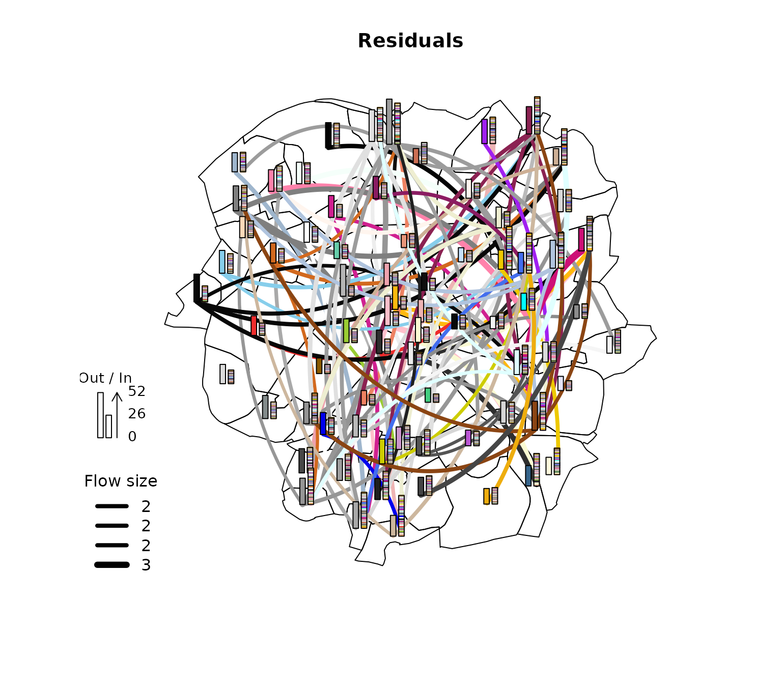
Looking at the relation between the distances and the error confirms
this impression. A more complex model could account for the increasing
variance by weighting the observations during the estimation. This could
be achieved using the weight_variable option in
spflow_control(), but is left out in this introductory
vignette.

Evaluating the impact of changing the input data
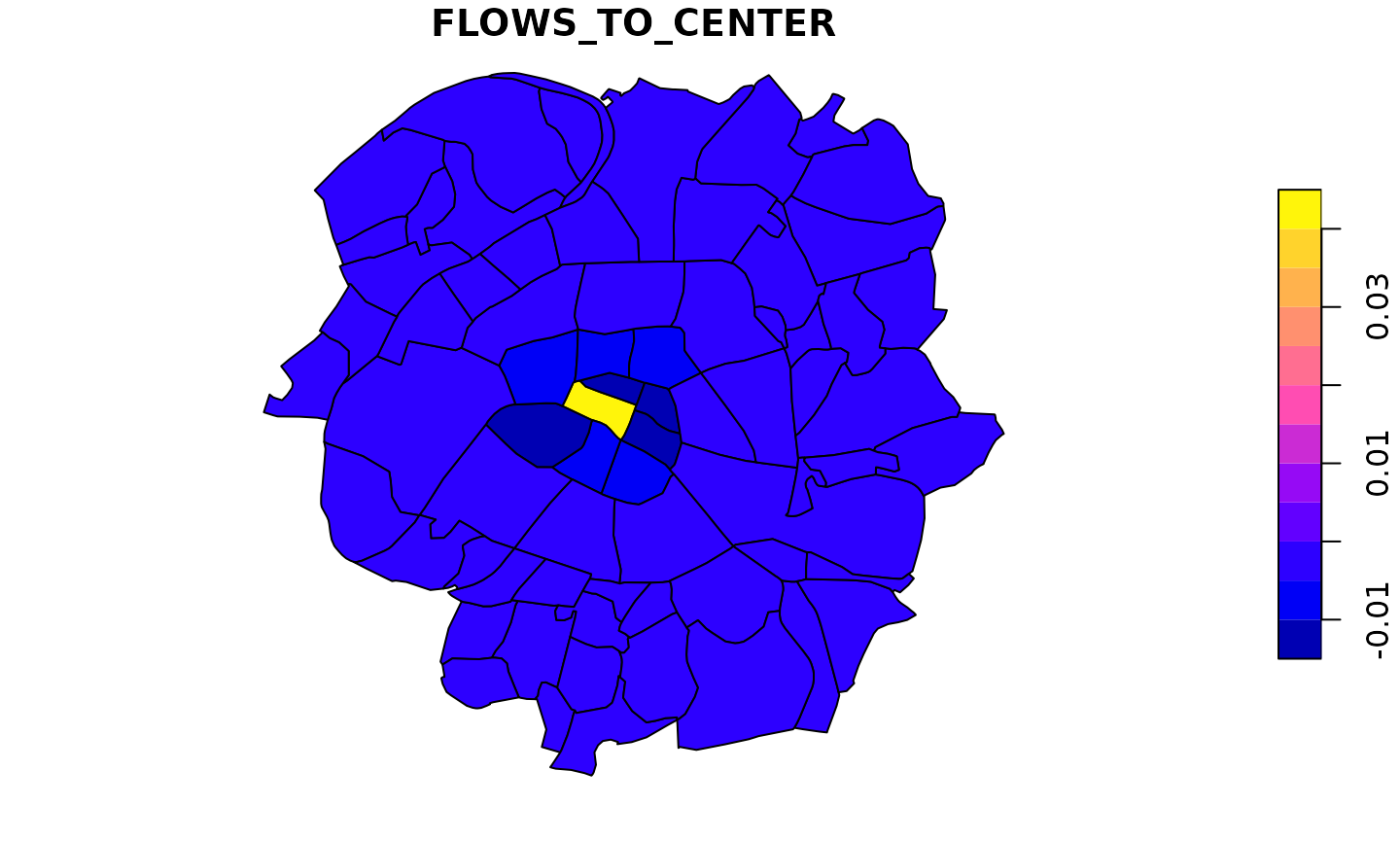
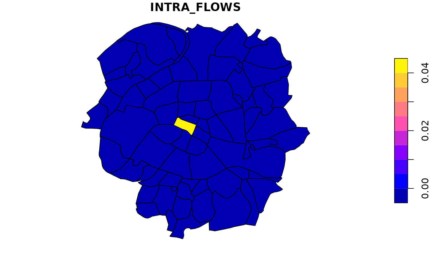
Finally we can evaluate the impact certain characteristics have on the outcome. Here we look at a scenario where the population in the central municipality is increased by 10%. As this has diverse effects on all flows we will first look at an image of the effect matrix. For a more detailed treatment of the effect decomposition in the spatial econometric interaction model see and .
center_mun <- "75101"
change_paris <- dat(paris10km_multinet, "paris")
change_paris <- change_paris[change_paris$ID_MUN == center_mun,]
change_paris[,"POPULATION"] <- change_paris[,"POPULATION"]*1.1
change_paris <- change_paris[,1:2] # keep the ID and the variable that changed

effect_matrix <- predict_effect(
  results_mcmc,                           # the model
  new_dat = list("paris" = change_paris), # changes in network "paris"
  return_type = "M")                      # return in matrix form


# in the first row are those flows that go to the center
# in the first column are those flows that start from the center
image(effect_matrix)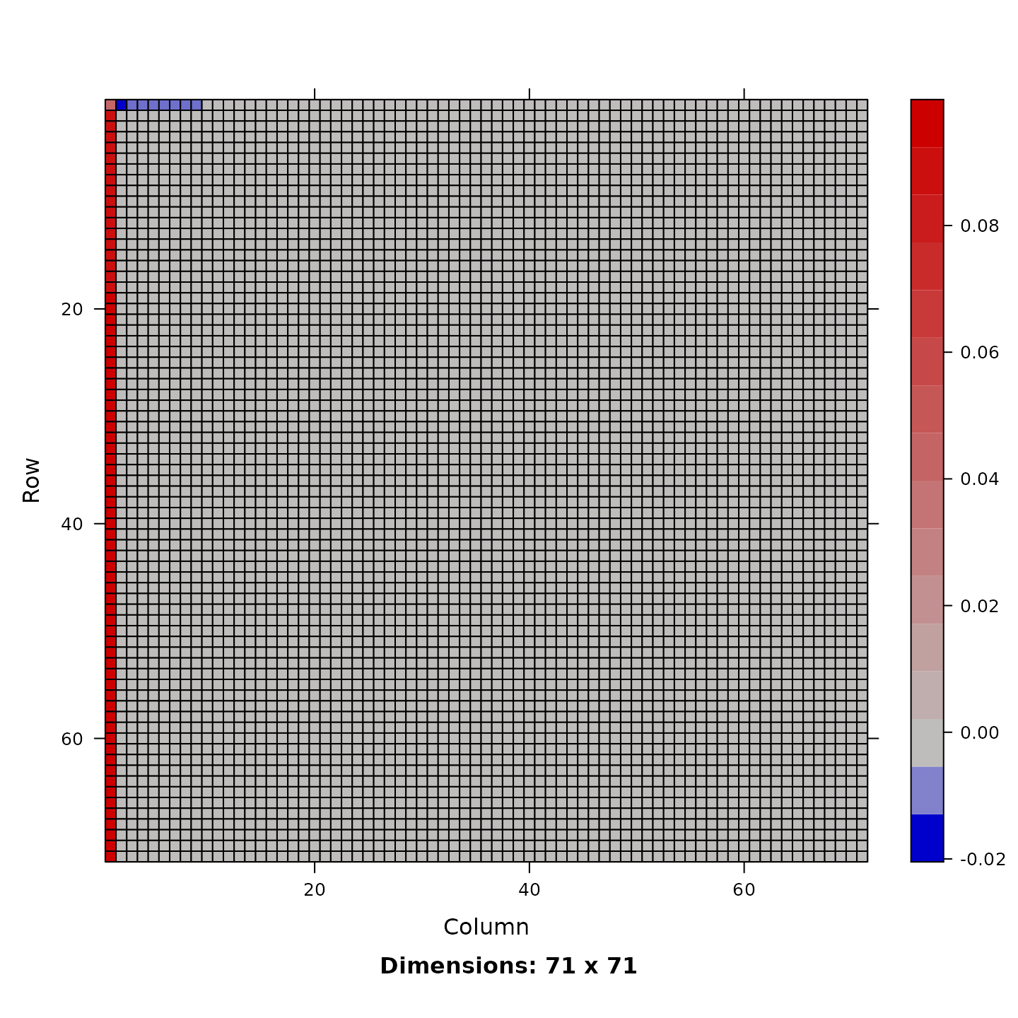
Here we see that flows starting from the center increase and flows that start from neighbors of the center to the center decrease. All other effects are very small. We can then have a closer look at the flows that start from the center or go to it. Additionally we look at all the internal flows, which decrease for all municipalities except for the center.
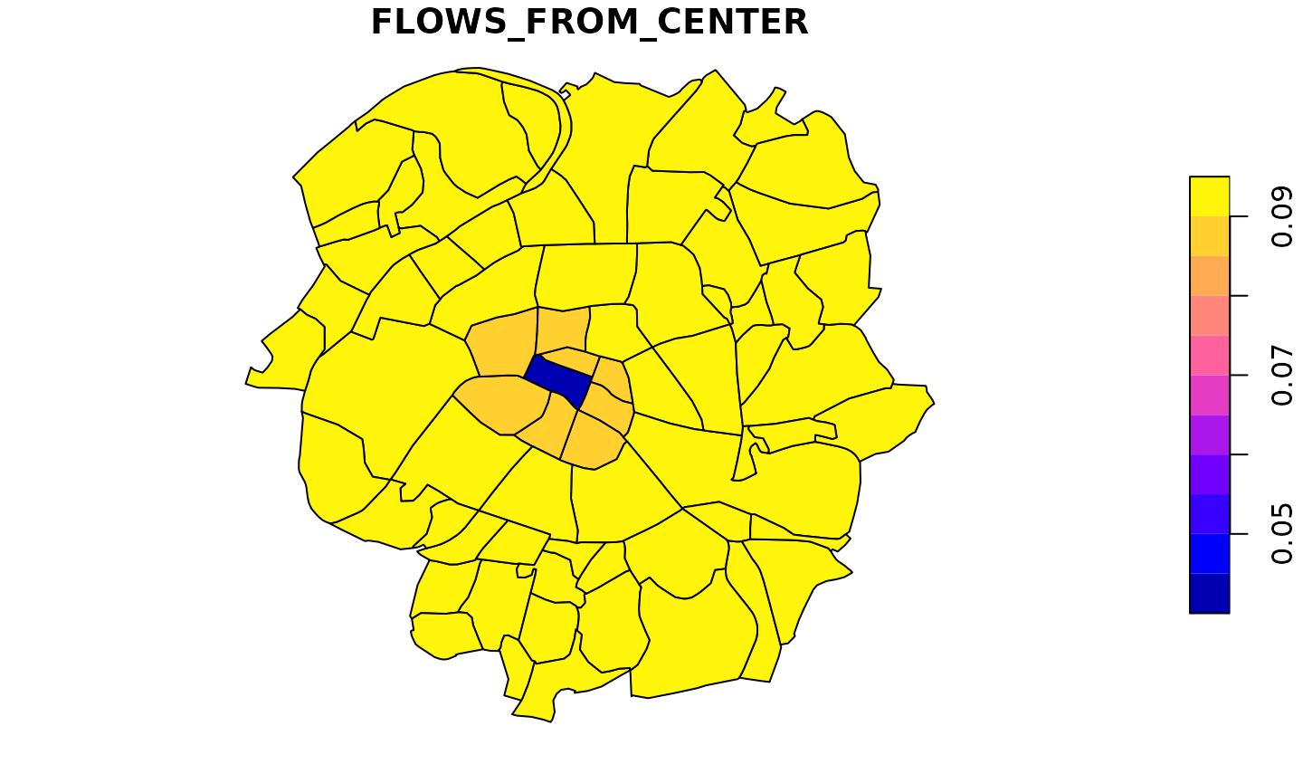
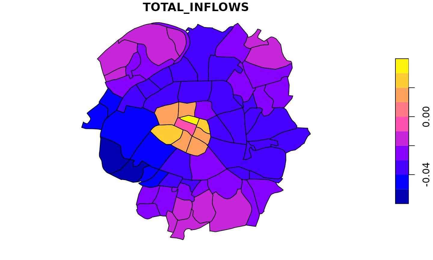
We can then look at the indirect effects on all flows that do not have the central municipality as origin or destination. To summarize these by total inflow and outflow we additionally set the internal flows to zero.
effect_matrix2 <- effect_matrix
diag(effect_matrix2) <- effect_matrix2[1,] <- effect_matrix2[,1] <- 0
plot(cbind("TOTAL_OUTFLOWS" = rowSums(effect_matrix2), paris10km_municipalities["geometry"]))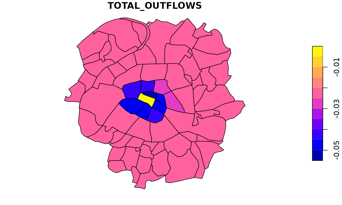
References
Dargel L, Thomas-Agnan C (2022). “A generalized framework for estimating spatial econometric interaction models.” TSE Working Paper, n. 22-1312, https://www.tse-fr.eu/publications/generalized-framework-estimating-spatial-econometric-interaction-models.
Goulard M, Laurent T, Thomas-Agnan C (2017). “About predictions in spatial autoregressive models: optimal and almost optimal strategies.” Spatial Economic Analysis, 304–325. https://doi.org/10.1080/17421772.2017.1300679.