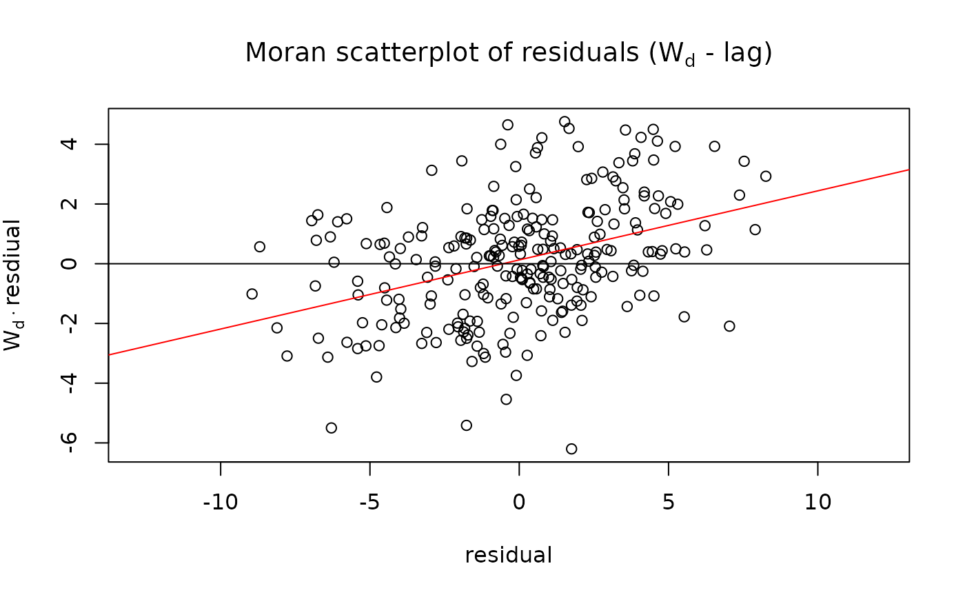
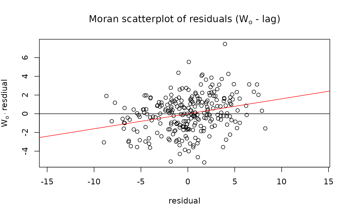
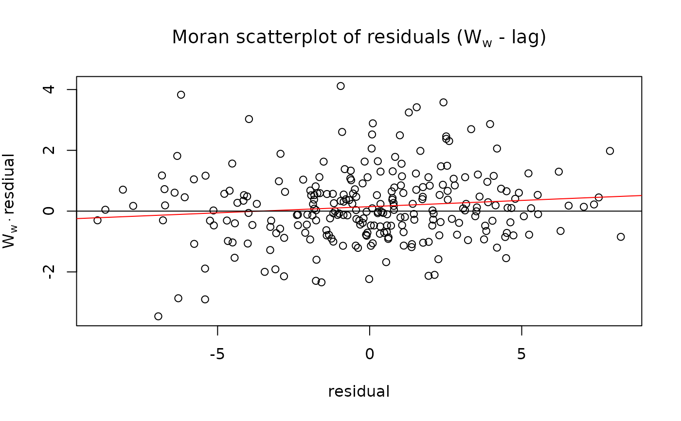
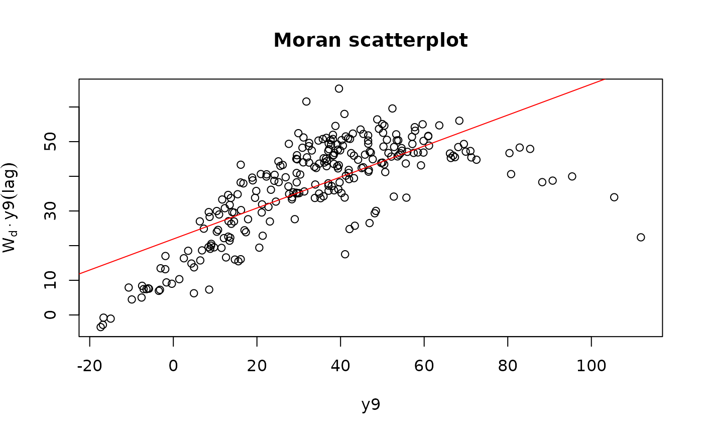
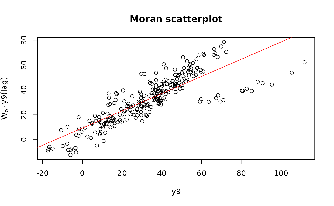
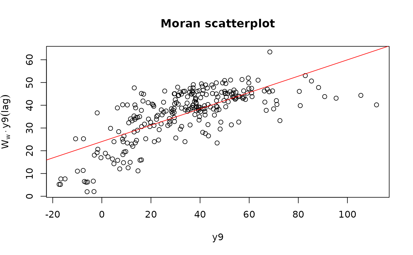
Moran scatter plots of interaction data

Generate up to three Moran scatter plots, related to origin-, destination-, and origin-to-destination-dependence.

spflow_moran_plots(object, ...)

# S4 method for spflow_network_multi
spflow_moran_plots(
  object,
  id_net_pair = id(object)[["pairs"]][[1]],
  flow_var,
  model = "model_9",
  DW,
  OW,
  add_lines = TRUE
)

# S4 method for spflow_model
spflow_moran_plots(object, model = "model_9", DW, OW, add_lines = TRUE)

Arguments

object

A spflow_network_multi-class() or a spflow_model-class()

...

arguments passed to methods

id_net_pair

A character indicating the id of a spflow_network_pair() (only relevant if the spflow_network_multi() contains multiple spflow_network_pair-objects: defaults to the of them)

flow_var

A character, indicating one variable from the network pair data

model

A character indicating the model number, that controls different spatial dependence structures should be one of paste0("model_", 1:9). Details are given in the documentation of spflow_control().

DW, OW

A matrix to replace the neighborhood of the destinations (DW) and origins (OW). Defaults to the one supplied to the model.

add_lines

A logical, if TRUE regression lines are added to the Moran scatter plots.

Examples

 # Used with a spflow_network_multi ...
 # To check the if there is spatial correlation in any variable
 spflow_moran_plots(multi_net_usa_ge, "ge_ge",flow_var = "y9")





 # Used with a spflow_model...
 # Check the if there is spatial correlation in the residuals
 gravity_ge <- spflow(
   y9 ~ . + P_(DISTANCE),
   multi_net_usa_ge,
   "ge_ge",
   spflow_control(model = "model_1"))

 spflow_moran_plots(gravity_ge)